Model schema and the simulation environment
The model simulation page loads with a schematic representation of the current model. A particular model’s simulation page can be accessed directly using the following URL structure:
http://jjj.bio.vu.nl/models/<model slug>/simulate/
e.g. for the teusink model:
- This page is where all of the available analyses are performed including:
The various analyses may be accessed using the navigation tabs just above the schema. Additionally, the model may be edited or downloaded using the Detail and Download buttons on the top-left of the page.
The Schema
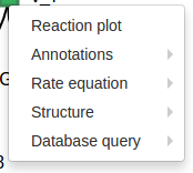
Models are represented by a dynamically-rendered schema consisting of reaction  and species
  nodes. Certain curated models have predefined schemas which are applied upon instantiation; other models are simply layed out using a forcing function. Right-clicking on these nodes will reveal a context menu containing links to respective reaction plot pages, annotations, rate equations, species structures, and external links to query the entity in either the BRENDA or SABIO-RK databases.

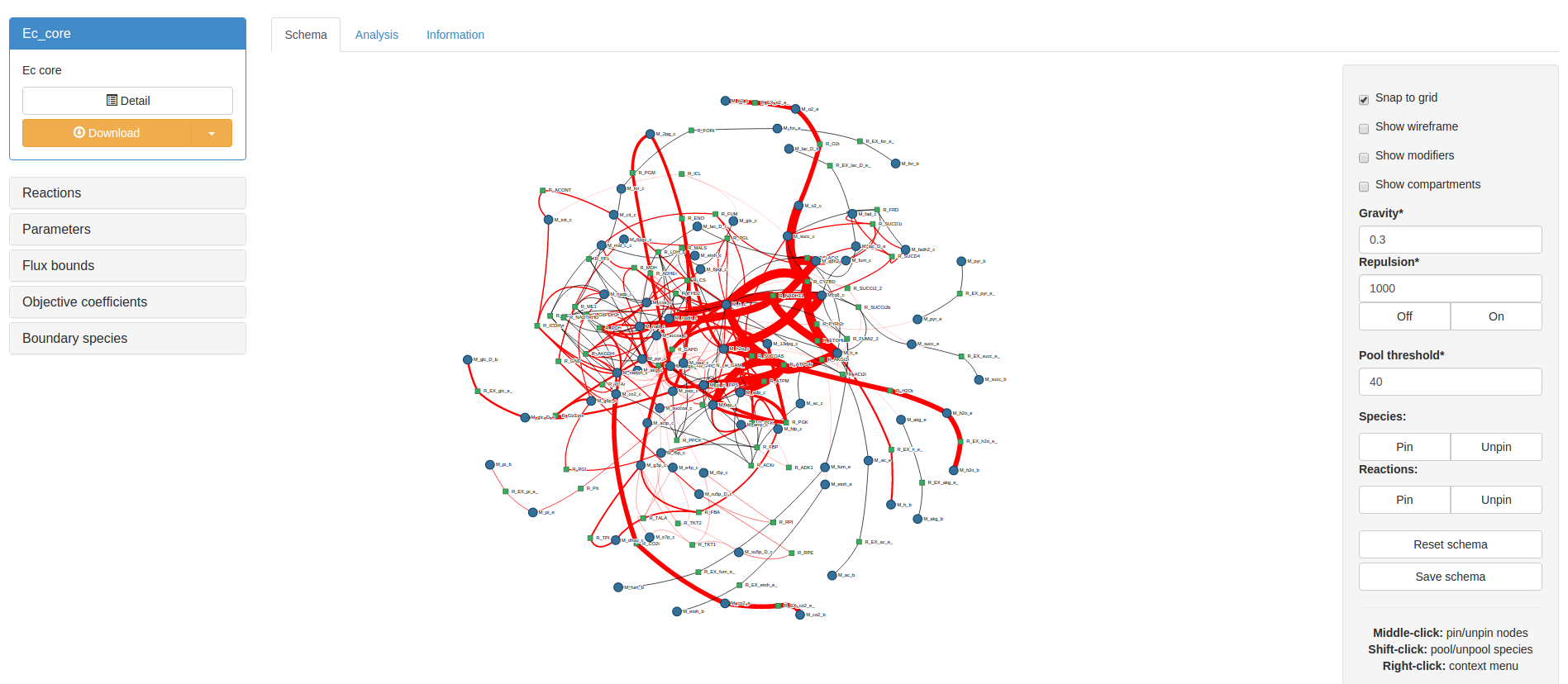
The model schema can be manipulated by dragging individual nodes with the mouse and by adjusting the schema settings in the box on the righthand side. A number of the less obvious options in this box are explained in the following section:
- Show modifiers: regenerate the schema showing allosteric effects as dashed lines
- Show compartments: plot convex hulls around nodes contained in various compartments
- Gravity: this value determines the degree to which nodes are attracted to the centre of the image
- Repulsion: this value determines the degree to which nodes repel each other
- Pool threshold: Large reaction networks often become convoluted and difficult to interpret, especially when certain species are involved in many reactions (e.g. cofactors like NADH, ATP). The schema algorithm automatically breaks species into multiple pooled species
if they take part in a certain number of reactions (determined by Pool threshold). Individual nodes can be pooled by shift-clicking. This will override the Pool threshold.
- Pin/Unping species and reaction: These options fix the position of all members of the respective node type. Individual nodes can be fixed by middle-clicking with a mouse.
Finally, if the model shares a number of node IDs with another model, an option exists to attempt to apply that model’s predefined layout to the current model. Obviously, this will only be successful if enough of the IDs are shared, and if the applied layout will sensibly transpose onto the current network.
Time evolution
Dynamic models (as opposed to contraint-based models) can be simulated over time by clicking on the Time evolution tab. To produce a time evolution plot, the species, reaction rates, and assignment rules to be plotted can be selected in the control box on the righthand side. Clicking ‘Go’ will perform the simulation and a new results panel will appear. The simulated values can be accessed as comma-separated values by clicking on the CSV button in the result panel:
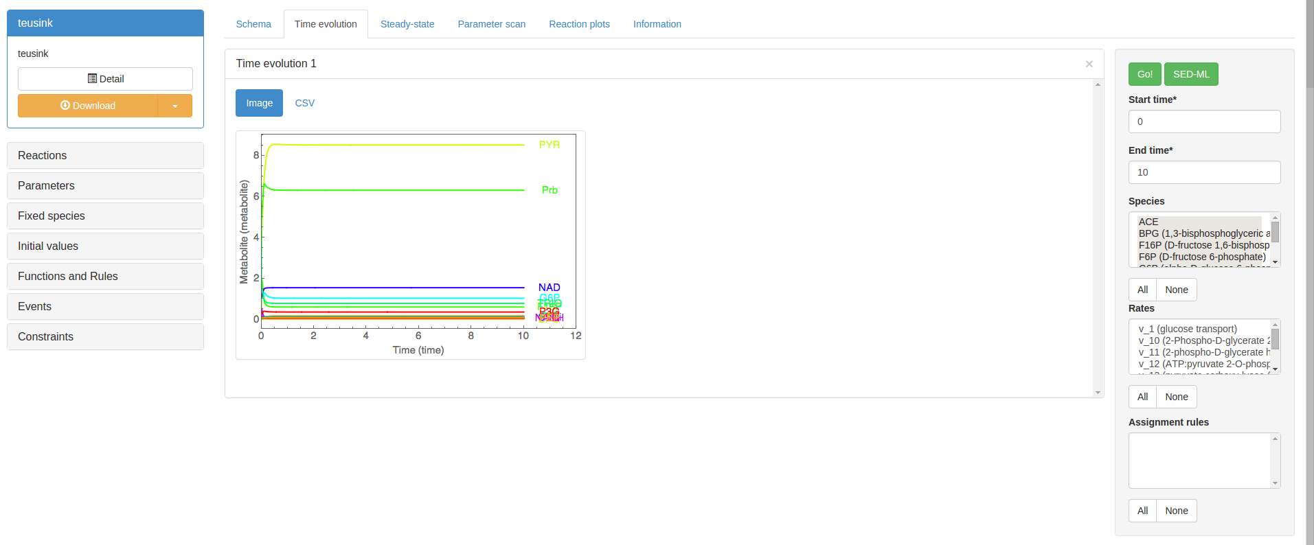
The accordion box on the lefthand side of the simulation page contains all the model features according to type. Changing a parameter value, for instance, will allow you to perform time evolutions with the new parameter value. This is only a temporary change. To make permanent model alterations use the model detail page accessed using the detail button on the top-left of the page.
Steady-state and Control Analysis
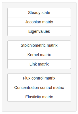
Clicking on the Steady-state tab will take you to the steady-state analysis page. The analysis options are contained in a control box on the righthand side of the page. Options include:
- Steady state: If the model is capable of achieving a steady-state flux (\(\frac{\partial \boldsymbol{s}}{\partial t} = \boldsymbol{0}\)) this button will return the steady-state concentrations and fluxes.
- Jacobian matrix: returns the matrix of all first-order partial derivatives of the system variables
- Eigenvalues: returns the eigenvalues of the Jacobian matrix
- Stoichiometric, Kernel, and Link matrices: return the respective structural matrix
Control Analysis is a framework for exploring the degree of control exercised by various elements in a dynamic model (see Kacser and Burns and Heinrich and Rapoport). Flux and concentration control coefficients, as well as elasticities are available as matrices using the last three buttons in the control box.
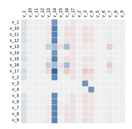
Note that all matrices can be viewed as rendered mathematical expressions, heat maps, or in .csv format. Below is an example of a heat map of the matrix of flux control coefficients for the teusink model (blue is positive, red is negative):
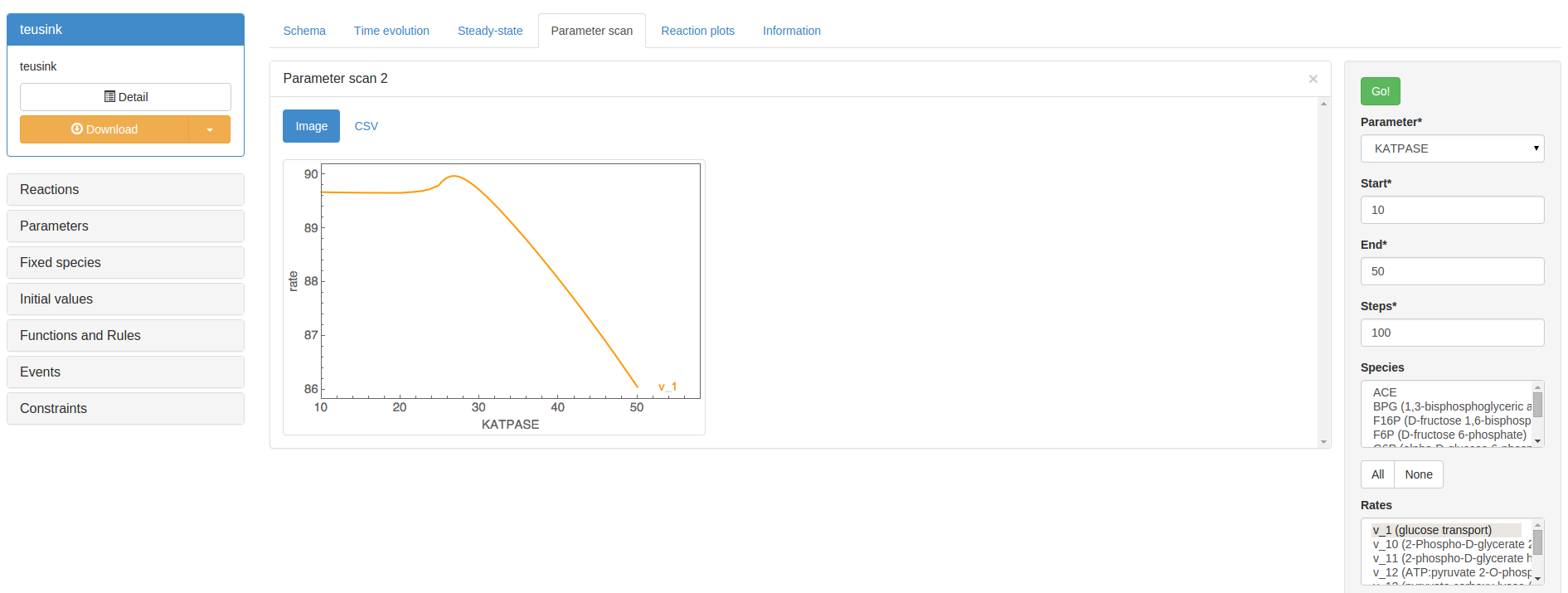
Parameter scanning
In the Parameter scan section, you are able to perform a scan of the effect of an individual model parameter on a selection of steady-state variables. In the control box on the right you will be able to specify a parameter to scan, the desired scan values (start, end, steps), and the output variables (Species, Rates, Assignment rules) to plot. Clicking ‘Go’ will perform the scan and display the results in a new result panel.
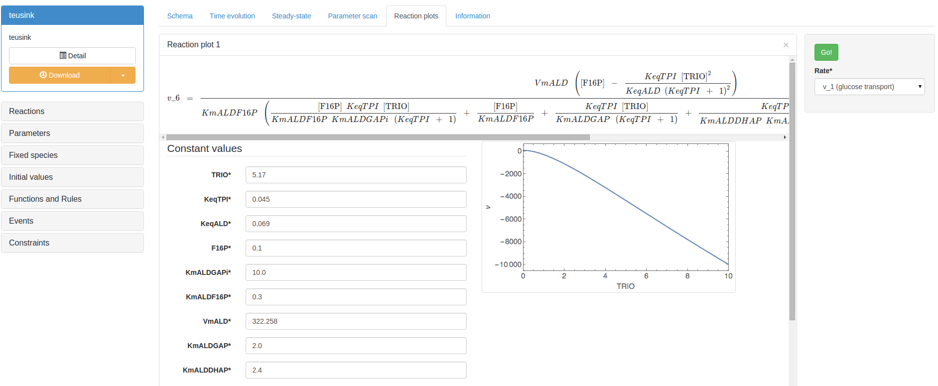
Reaction plot
In the Reaction plot section, you are able to plot the effect of changing individual variables or parameters on the rate of an individual reaction in isolation from the rest of the system (i.e. a local rather than systemic effect). First, a rate must be selected in the drop-down list in the righthand control box. The reaction of interest will be displayed in its own result panel, including a rate equation and all associated variables and parameters. Setting all parameter/variable values, and the scan range values, and then clicking ‘Go’ in the panel will perform a reaction plot:
RESTful reaction plots
For ease of access, reaction plots may be performed directly by constructing an appropriate URL. The URL must refer to the desired model and contain certain GET parameters. For example, the URL linking to the teusink model (see Model schema and the simulation environment):
http://jjj.bio.vu.nl/models/teusink/simulate/
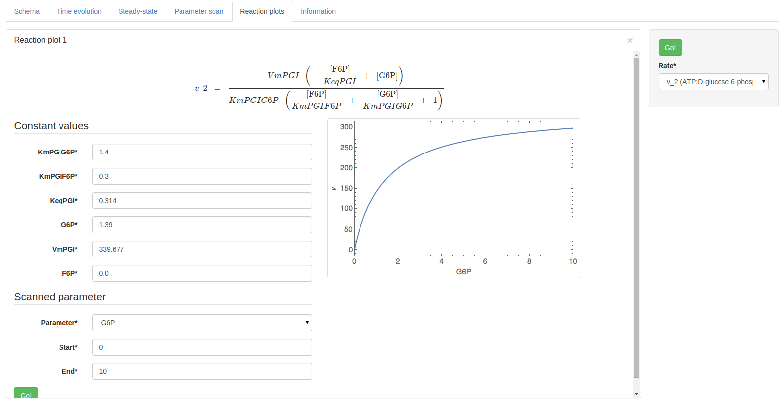
Can be modified with some parameters to automatically perform a reaction plot:
http://jjj.bio.vu.nl/models/teusink/simulate/?rateplot=v_2;parameter=G6P;F6P=0.0
- rateplot=v_2 - this specifies the reaction with which to perform the reaction plot, in this case v_2
- parameter=G6P - this specifies which parameter/variable to scan, in this case G6P
- F6P=0.0 - the remainder of the parameter and variable values may be set, in this case only F6P is given a value
Using the constructed URL above will produce the following result page:
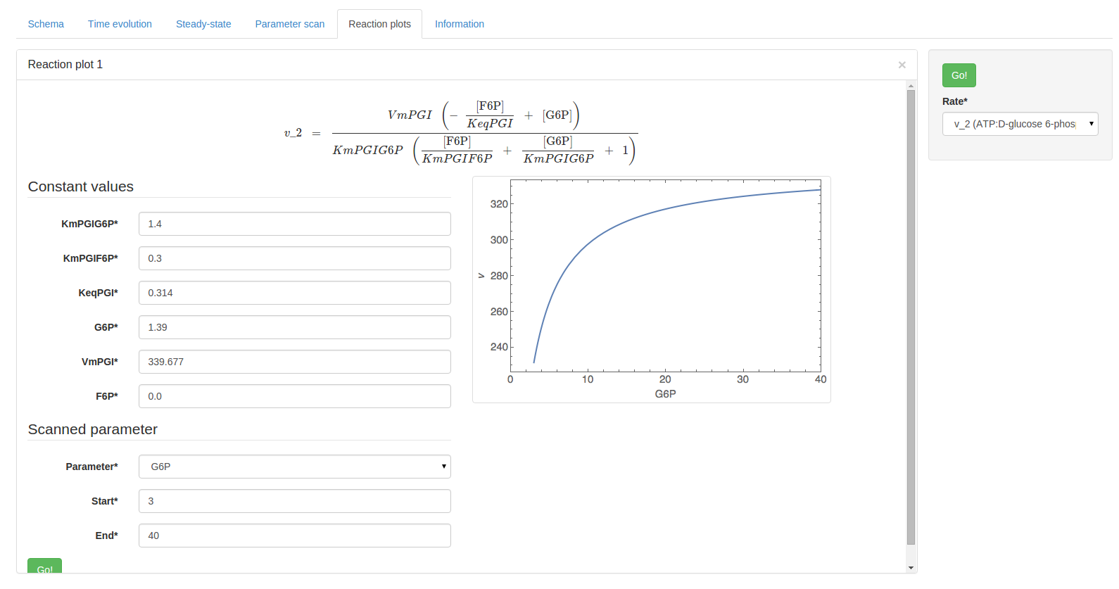
Additionally, the start and end parameters determine the scan range:
Flux Balance Analysis
Finally, if the model being analysed is a constraint-based model (lacking kinetics), a Flux Balance Analysis may be performed. In fact, during the upload process a user may specify that the model being uploaded should be treated as a constraint-based model and kinetics will be ignored:
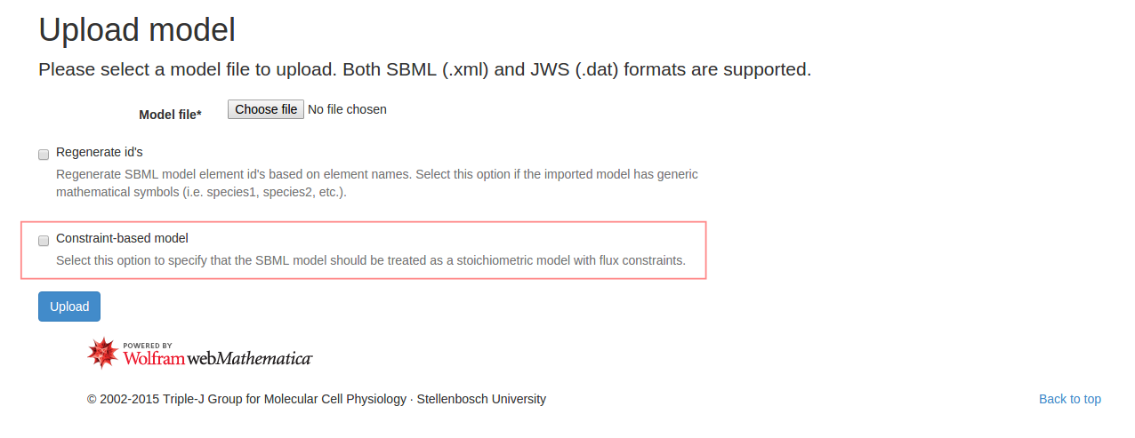
In this case a set of generic flux bounds will be applied. Using a contraint-based models on JWS Online will produce a significantly reduced user interface, with all the dynamic analyses removed. Flux Balance Analysis may be performed by navigating to the Analysis tab, and clickin the Flux Balance Analysis button in the righthand control box. If appropriate objectives have been specified, a result panel will appear with the optimised flux solution:
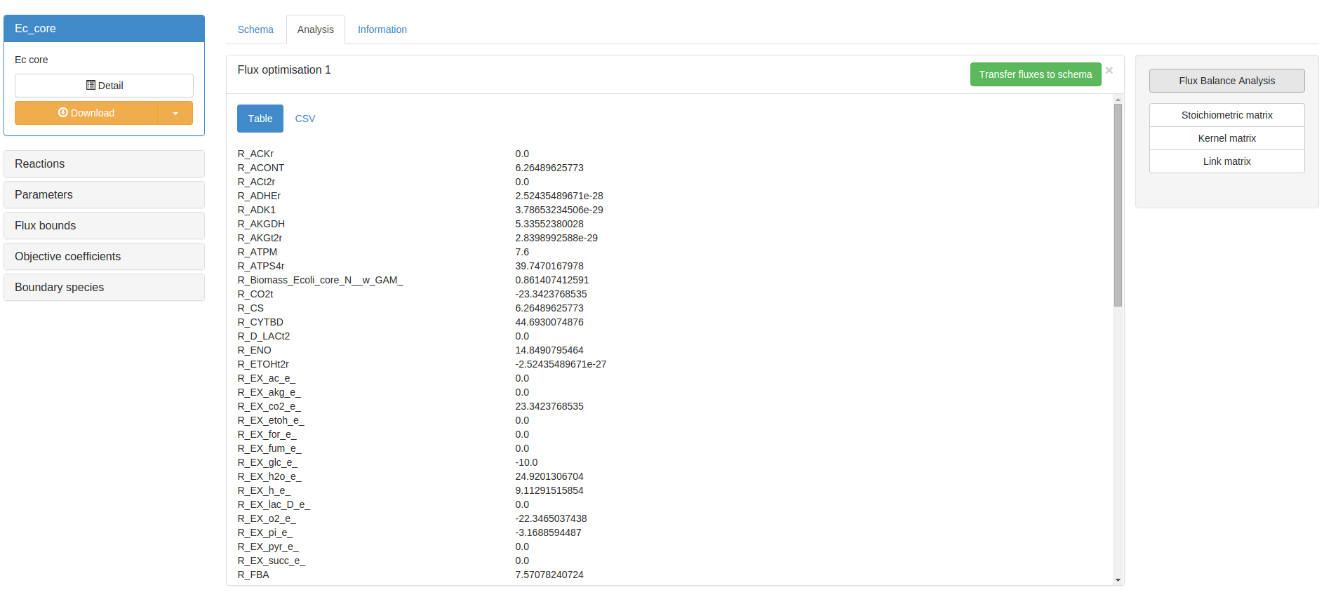
Before optimising flux, bounds and objectives may be temporarily edited using the accordion box on the lefthand side of the screen. Lastly, any particular flux solution may be transferred to the schema by clicking the Transfer fluxes to schema button in the result panel. This will map the flux solution onto the schema in various thicknesses of red reaction lines. Black lines represent a flux of 0:
RESTful FBA
Flux Balance Analyses may be performed directly by contructing a specific URL. For example, the following URL links directly to the result of an FBA on the Orth1 model by simply specifying the fba parameter as true:
Adding the transfer_fluxes=true flag will link directly to a schema with flux overlay: